

결정 경계를 정의하는 데 필요한 데이터들이 서포트 벡터뿐이기 때문에 나머지 데이터들은 무시해도 된다. 따라서 매우 빠르게 처리 가능
앙상블
: 여러 개의 분류기를 합친다는 의미로써의 모델. 약한 분류기들을 합쳐 더 좋은 예측을 하기 위해 만들어짐.
학습 유형
•
보팅
•
배깅
•
부스팅
보팅?
서로 다른 알고리즘을 가진 모델을 결합한 모델
배깅?
같은 알고리즘을 가진 모델을 데이터 샘플링을 다르게 하여 학습하는 모델
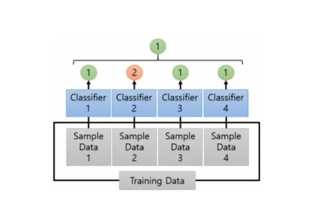
하드보팅 VS 소프트보팅
•
하드 보팅 : 다수결원칙. 다수의 분류기가 예측한 값을 최종 결괏값으로 선정
•
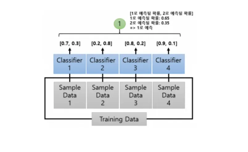
소프트 보팅 : 분류기들의 예측확률의 평균으로 결괏값을 선정
배깅
학습데이터에서 일부가 중첩되게 샘플링하여 서로 다른 데이터 세트를 만드는 방식을 사용하는데 이를 부트스트래핑 분할 방식이라고 부른다.
배깅 - 랜덤포레스트
여러 개의 결정 트리 분류기를 결합해 보팅을 통해 최종 예측 결과를 결정함.
랜덤포레스트의 하이퍼 파라미터 및 튜닝
•
n_estimators : 결정 트리(즉, 약한 분류기)의 갯수를 지정, 디폴트는 10
•
max_features : 결정 트리의 max_features와 같음. 하지만 디폴트는 sqrt(=auto)
그외 다수는 결정 트리의 하이퍼 파라미터와 동일함. (생략)
부스팅
여러 개의 학습기를 순차적으로 학습/예측 해나가면서 잘못 예측한 데이터에 가중치를 부여해 오류를 개선해나가는 방식.
대표적인 방법은
•
adaboost
•
그래디언트부스트
부스팅 - GBM(Gradient Boosting Machine)
오차의 가중치 업데이트를 경사 하강법을 사용하는 모델
but 단점 : 수행시간이 오래 걸리고, 하이퍼 파라미터 튜닝의 수고가 필요함.
< GBM의 하이퍼 파라미터 >
•
loss(default=’deviance’) : 경사 하강법에서의 비용 함수
•
learning_rate(default=0.1) : 작을수록 예측 성능 좋아지지만 오래 걸린다.
•
n_estimators(default=100) : 하위 모델의 갯수
•
subsample(default=1) : 학습에 사용할 데이터 샘플링의 비율. 과적합이 염려될 경우 1보다 작은 값으로 지정
XGBoost
GBM을 개선시킨 모델. GBM의 느린 학습 수행 속도와 과적합 규제 부재등을 해결한 모델이다.
< 패키지 모듈 >
•
파이썬 래퍼 XGBoost 모듈
•
사이킷런 래퍼 XGBoost 모듈
—> 둘의 하이퍼 파라미터 차이가 존재하기 때문에 유의해야 한다. 하지만 일반적으로 사이킷런 래퍼를 많이 사용!
LightGBM
XGBoost를 또다시 개선시킨 모델. 시간과 용량을 모두 단축시켰다. 예측 성능에는 큰 차이가 없다.
but 단점 : 적은 데이터 세트(10,000건 이하)를 적용하면 과적합이 발생하기 쉽다.
특징 : 다른 결정 트리 분할 방식과 달리 리프 중심 분할 방식
장점 :
< LightGBM의 하이퍼 파라미터 >
•
주요 파라미터
◦
n_estimators(default=100)
◦
learning_rate(default=0.1)
◦
max_depth(default=-1)
◦
min_child_samples(default=20)
◦
num_leaves(default=31)
◦
boosting(default=gbdt)
◦
subsample(default=1)
◦
colsample_bytree(default=1)
◦
reg_lambda(default=0) : l2 regulation
◦
reg_alpha(default=0) : l1 regulation
•
학습 태스크 파리미터
◦
objective : 손실함수
SVM(서포트 벡터 머신)
: 분류모델 중 하나.
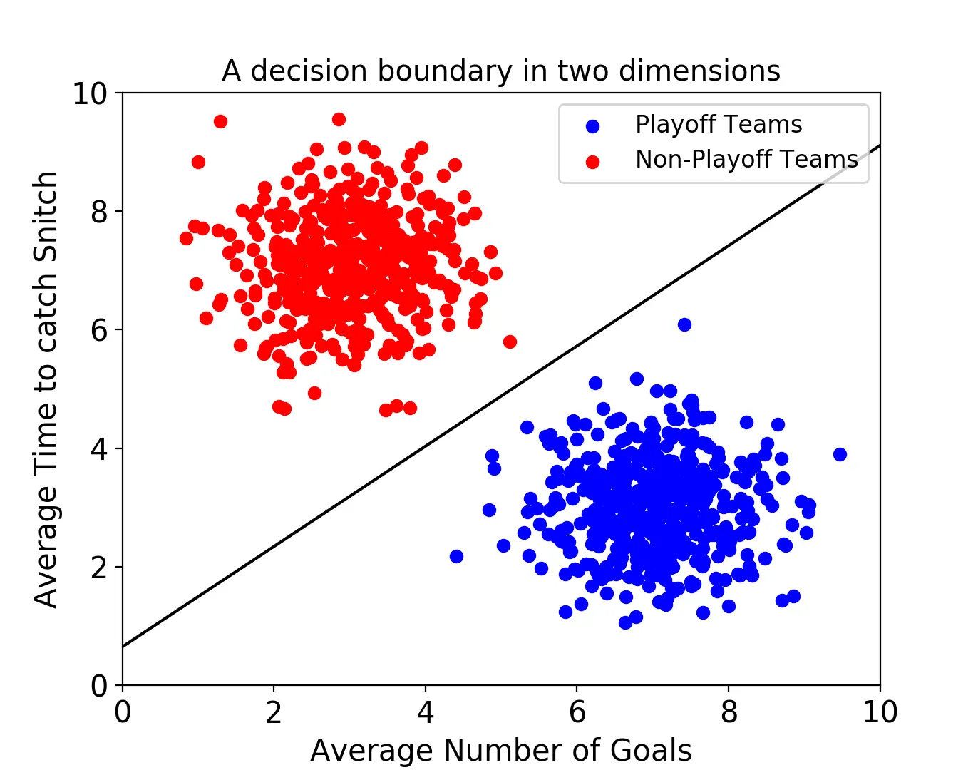
서포트 벡터 머신은 결정 경계(Decision Boundary) , 즉 분류를 위한 기준 선을 정하는 모델이다.
속성이 2개인 데이터 : 결정 경계는 아래처럼 2차원의 선으로 표현됨.
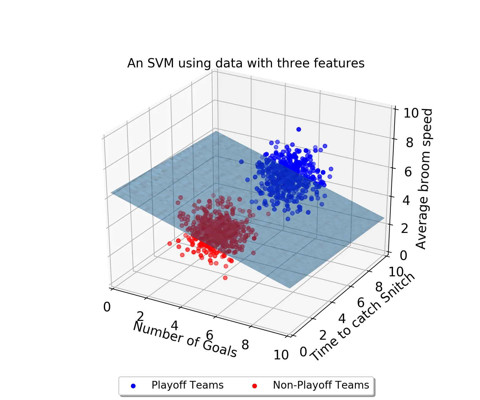
속성이 3개인 데이터 : 3차원으로 표시되고 결정 경계는 평면으로 표현됨.
속성이 4개 이상인 데이터 : 고차원으로 넘어가기 때문에 형성되는 결정 경계를 초평면이라고 부름.
최적의 결정 경계
최적의 결정 경계를 찾는 것이 목표가 된다.
HOW?
결정 경계는 데이터 군으로부터 최대한 멀리 떨어지는 것이 좋다.
support vectors : 결정 경계와 가장 가까이 있는 데이터들
→ 결정 경계를 정의하는 가장 결정적인 역할
마진
: 결정경계와 서포트 벡터 사이의 거리
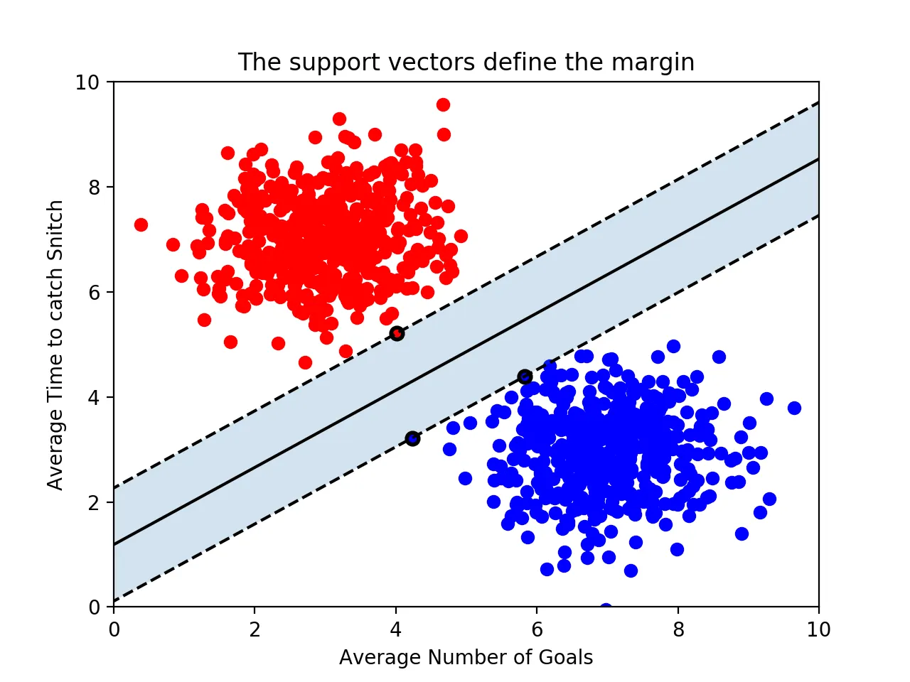
따라서 마진을 최대화하는 결정 경계가 최적의 결정 경계가 된다.
BUT 유의할 점 : n개의 속성을 가진 데이터에는 최소 n+1개의 서포트 벡터가 존재해야 한다
SVM 의 장점 :
•
결정 경계를 정의하는 데 필요한 데이터들이 서포트 벡터뿐이기 때문에 나머지 데이터들은 무시해도 된다. 따라서 매우 빠르게 처리 가능
•
회귀와 분류 문제에 적용 모두 가능
•
예측력이 좋다.
SVM의 단점:
•
해석이 어렵다.
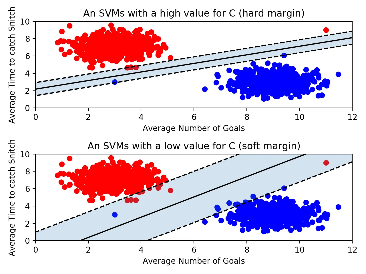
이상치의 허용
•
하드 마진 : 아웃라이어를 허용하지 않는 기준으로 빡세게 결정 경계를 정의
→ 마진이 매우 좁아지고 과적합의 위험이 있음.
•
소프트 마진 : 아웃라이어를 마진 안에 허용함으로써 기준을 넉넉히 정의하는 것
→ 마진이 커지게 되지만 언더피팅의 위험이 있음.
Scikit-learn 에서의 SVM
from sklearn.svm import SVC
classifier = SVC(kernel='linear')
training_points = [[1, 2], [1, 5], [2, 2], [7, 5], [9, 4], [8, 2]]
labels = [1, 1, 1, 0, 0, 0]
classifier.fit(training_points, labels) # 학습
classifier.predict([[3,2]]) # 예측
classifier.support_vectors_ #결정 경계를 정의하는 서포트 벡터
SQL
복사
하이퍼 파라미터 C
C(default=1) : 이상치 허용 파라미터.
→ C값이 클수록 하드마진, 작을수록 소프트 마진이다.
sol) C의 최적 값은 GridSearchCV를 통해서 찾아나간다.
classifier = SVC(C=0.01)
SQL
복사
kernel
결정 경계를 선, 곡선, rbf 등으로 구체적으로 지정
classifier = SVC(kernel='poly')
SQL
복사
BUT 주의해야 할 점 : 단순히 이상치때문에 선형으로 분리할 수 없다고 판단해서 선형 아닌 커널을 사용하면 안된다. —> 과적합의 위험
•
poly(다항식) :
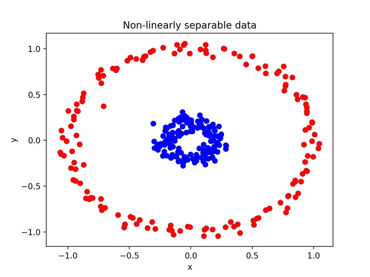
•
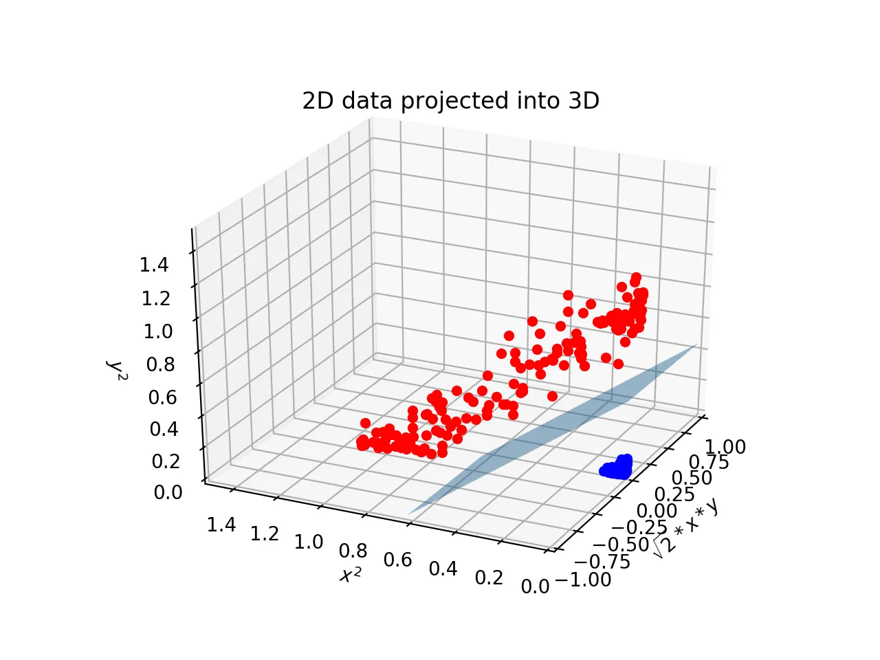
rbf(방사 기저 함수) : RBF커널 혹은 가우시안 커널, kernel의 기본값
→ 2차원의 점을 무한한 차원의 점으로 변환
classifier = SVC() # default kernel = 'rbf'
SQL
복사
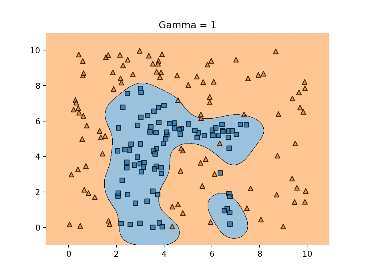
하이퍼 파라미터 감마
학습 데이터에 얼마나 민감하게 반응할 것인지를 조정해주는 것으로 C와 비슷
classifier = SVC(C=2, gamma=0.5)
SQL
복사
gamma↑ : 과적합 위험↑
gamma↓ : 언더피팅의 위험↑
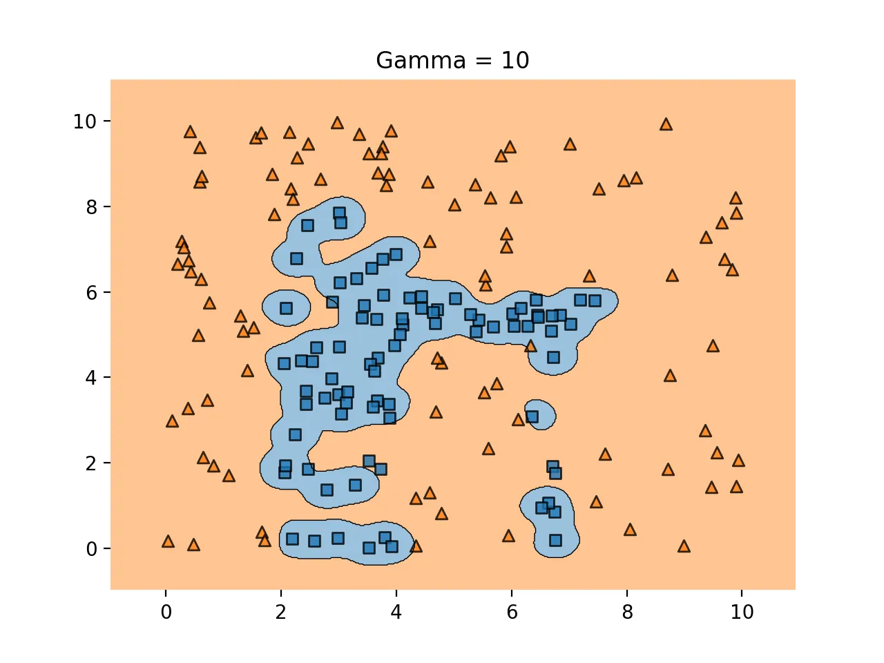
과적합의 예시
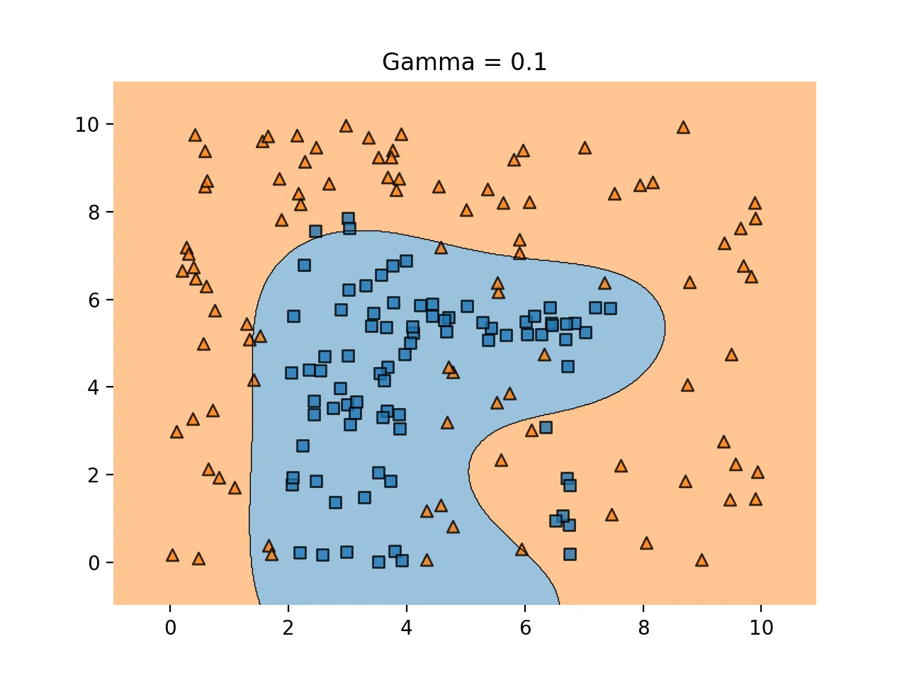
언더피팅의 예시
scikit-learn 붓꽃 문제 적용
from sklearn.datasets import load_iris
iris = load_iris()
x1 = iris.data[:100,:2] # 100개의 데이터와, 2개의 변수만 활용
y1 = iris.target[:100] # 종속변수
from sklearn.svm import SVC
model1 = SVC(kernel='linear', C=1e10).fit(x1,y1) # C값이 10의 10승이므로 매우 큰 값. 하드마진 서포트벡터
# 예측 결과의 평가
from sklearn.metrics import classification_report
print(classification_report(y1,model1.predict(x1)))
# 결과
precision recall f1-score support
0 1.00 1.00 1.00 50
1 1.00 1.00 1.00 50
accuracy 1.00 100
macro avg 1.00 1.00 1.00 100
weighted avg 1.00 1.00 1.00 100
# 이번에는 C값을 0.1로 지정하여 다시 구해보자.
model2 = SVC(kernel='linear', C=0.1).fit(x1,y1)
print(classification_report(y1,model2.predict(x1)))
SQL
복사
stroke 데이터 문제 적용
import numpy as np
import pandas as pd
import matplotlib.pyplot as plt
import seaborn as sns
sns.set_style('whitegrid')
# load data
df = pd.read_csv('D:me/jupyterNotebook/study/strokedata.csv')
df.drop('id', axis=1,inplace=True)
df.head()
df.info()
df.describe()
###### data cleansing ######
# dealing with na
# 'bmi' 열의 null값을 mean으로 대체
df['bmi'] = df['bmi'].fillna(df['bmi'].mean())
# 'gender'내의 Other값을 가지고 있는 행 제거
other_index = df[df['gender']=='Other'].index
df = df.drop(other_index)
###### visualizing features ######
# 흡연여부, 직장, 거주지역이 stroke와의 연관성이 있을까?
# 확인해보기 위해 시각화를 진행한다.
import warnings
warnings.filterwarnings('ignore')
plt.figure(figsize=(21,5))
# 흡연여부 그래프 (stroke에 대한)
plt.subplot(1,3,1) # subplot 중 첫번째
sns.countplot(x=df['smoking_status'], alpha=0.8, palette='Paired', hue=df['stroke']);
sns.despine(fig=None, ax=None, top=True, right=True, left=False, bottom=True, offset=None, trim=False);
plt.xlabel('');
plt.title('Smoking Status');
# 직장 타입
plt.subplot(1,3,2)
sns.countplot(x=df['work_type'], alpha=0.8, palette='Paired', hue=df['stroke']);
sns.despine(fig=None, ax=None, top=True, right=True, left=False, bottom=True, offset=None, trim=False);
plt.xlabel=('');
plt.title('Work Type');
# 거주 지역
plt.subplot(1,3,3)
sns.countplot(x=df['Residence_type'], alpha=0.8, palette='Paired', hue=df['stroke']);
sns.despine(fig=None, ax=None, top=True, right=True, left=False, bottom=True, offset=None, trim=False);
plt.xlabel=('');
plt.title('Residence Type');
--> 그림으로써는 큰 영향이 있는 것으로 판단되지 않는다.
#성별, 고혈압의여부, 심장병의 여부 가 stroke와의 연관성이 있을까?
plt.figure(figsize=(21,5))
plt.subplot(1,3,1)
sns.countplot(x=df['gender'], alpha=0.8, palette='Paired',hue=df['stroke']);
plt.tick_params(axis='both', which='both',bottom=False, left=True, right=False, top=False, labelbottom=True, labelleft=True); # 틱과 경계선을 한꺼번에 설정
sns.despine(fig=None, ax=None, top=True, right=True, left=False, bottom=True, offset=None, trim=False);
plt.xlabel=('')
plt.title('Gender, F/M : 59/41 %');
plt.subplot(1,3,2)
sns.countplot(x=df['hypertension'], alpha=0.8, palette='Paired',hue=df['stroke']);
sns.despine(fig=None, ax=None, top=True, right=True, left=False, bottom=True, offset=None, trim=False);
plt.xlabel=('')
plt.title('Hypertension');
plt.subplot(1,3,3)
sns.countplot(x=df['heart_disease'], alpha=0.8, palette='Paired',hue=df['stroke']);
sns.despine(fig=None, ax=None, top=True, right=True, left=False, bottom=True, offset=None, trim=False);
plt.xlabel=('');
plt.title('Heart Disease');
# 나이, 평균 Glucose level, bmi 가 stroke와의 연관성이 있을까?
sns.set_style('white')
plt.figure(figsize=(21,5))
plt.subplot(1,3,1)
sns.kdeplot(x=df['age'], alpha=0.2, palette='Set1', label='Smoker', fill=True, linewidth=1.5, hue=df['stroke']);
sns.despine(fig=None, ax=None, top=True, right=True, left=True, bottom=True, offset=None, trim=False);
plt.xlabel('');
plt.title('Age Distribution');
plt.subplot(1,3,2)
sns.kdeplot(x=df['avg_glucose_level'], alpha=0.2, palette='Set1', label='avg_glucose_level', linewidth=1.5, fill=True, hue=df['stroke']);
sns.despine(fig=None, ax=None, top=True, right=True, left=True, bottom=True, offset=None, trim=False);
plt.xlabel('');
plt.title('Average Glucose Level');
plt.subplot(1,3,3)
sns.kdeplot(x=df['bmi'], alpha=0.2, palette='Set1', label='BMI', shade=True, linewidth=1.5, hue=df['stroke']);
sns.despine(fig=None, ax=None, top=True, right=True, left=False, bottom=True, offset=None, trim=False);
plt.xlabel('')
plt.title('BMI');
SQL
복사
→ age가 확실히 영향력있는 변수인 것으로 확인된다.
# stroke 종속변수의 불균형적인 분포를 확인 --> 후에 오버샘플링이 필요
df['stroke'].value_counts()
SQL
복사
###### preprocessing data ######
# 범주형 데이터 --> 수치화
df['gender'] = df['gender'].replace({'Male':0, 'Female':1, 'Other':-1}).astype(np.uint8)
df['Residence_type'] = df['Residence_type'].replace({'Rural':0, 'Urban':1}).astype(np.uint8)
df['work_type'] = df['work_type'].replace({'Private':0, 'Self-employed':1, 'Govt_job':2, 'children':-1, 'Never_worked':-2}).astype(np.uint8)
df['ever_married'] = df['ever_married'].replace({'Yes':1, 'No':0}).astype(np.uint8)
df['smoking_status'] = df['smoking_status'].replace({'never smoked':0, 'Unknown':1, 'formerly smoked':2, 'smokes':-1}).astype(np.uint8)
SQL
복사
###### Model building #######
X = df.drop('stroke', axis=1)
y = df.pop('stroke')
# using SVM Classifier
# using pipeline
from sklearn.svm import SVC
from sklearn.pipeline import Pipeline
from sklearn.preprocessing import StandardScaler, LabelEncoder
svm_pipeline = Pipeline(steps=[('scale'.StandardScaler()), ('SVM',SVC(random_state=0. probability = True))])
SQL
복사
from sklearn.model_selection import train_test_split
X_train, X_test, y_train, y_test = train_test_split(X,y) # default
y_train.shape
# using SMOTE for oversampling
from imblearn.over_sampling import SMOTE
oversample = SMOTE()
X_train_resh, y_train_resh = oversample.fit_resample(X_train,y_train.ravel())
SQL
복사
교차 검증을 수행한다. cv=10 으로 우선 적용한다. 평가 지표는 f1 score로 진행한다.
from sklearn.model_selection import cross_val_score
svm_cv = cross_val_score(svm_pipeline, X_train_resh, y_train_resh, cv=10, scoring='f1')
svm_cv.mean()
###### model evaluation ######
from sklearn.metrics import confusion_matrix
svm_pipeline.fit(X_train_resh, y_train_resh);
svm_train_predict = svm_pipeline.predict(X_train)
svm_pred = svm_pipeline.predict(X_test)
svm_cm = confusion_matrix(y_train,svm_train_predict) # train데이터에 대한 오차행렬
from sklearn.metrics import roc_curve, auc
fpr_lr, tpr_lr = roc_curve(y_test, svm_pipeline.predict_proba(X_test)[:,1]) # test데이터에 대한 roc_curve
plt.figure(figsize=(12,8));
plt.plot(fpr_lr, tpr_lr);
plt.xlabel('False Positive Raet', fontsize=16);
plt.ylabel('True Positive Rate', fontsize=16);
plt.title('ROC curve', fontsize=16);
plt.plot([0,1],[0,1], color='navy', lw=3, linestyle='--');
sns.despine(fig=None, ax=None, top=True, right=True, left=False, bottom=False, offset=None, trim=False);
print('Auc : ', auc(fpr_lr, tpr_lr))
from sklearn.metrics import classification_report
from sklearn.metrics import accuracy_score, f1_score
print(classification_report(y_test,svm_pred))
print('Accuracy Score : ', accuracy_score(y_test,svm_pred))
print('F1 Score : ', f1_score(y_test,svm_pred))
SQL
복사
###### Grid Search Tunning ######
from sklearn.model_selection import GridSearchCV
param_grid = {'C':[0.1,1,10,1000], 'gamma':[1,0.1,0.01,0.001]}
grid = GridSearchCV(SVC(), param_grid, verbose=3)
# fit the data
grid.fit(X_train_resh,y_train_resh)
# best parameters based on param grid
grid.best_params_
# grid_model with best parameters
grid.best_estimator_
grid_train_predict = grid.predict(X_train)
grid_pred = grid.predict(X_test)
# evaluation of grid
classification_report(y_test,grid_pred)
classification_report(y_train,grid_train_predict)
SQL
복사