
모델의 일반화 성능을 높이기 위해서, 그리고 예측 정확도를 높이기 위해서는 피처 선택이 도움이 될 수 있다.
다음과 같은 경우에, 피처 선택이 필요할 수 있다.
1.
피쳐 수가 많을 때
피처가 많을 때는 타겟 변수와 상관이 없는 피처들이 많을 가능성이 높다.
이런 피처들은 없애주는 것이 성능 높이는 데 도움이 될 수 있다.
2.
피처 간 높은 상관관계가 있을 때
다중 공선성의 문제를 낳기 때문에 중복되는 피처가 있을 경우, 하나는 제거해주는 것이 좋다.
3.
노이즈 피처가 있을 때
타겟 변수와 관련 없거나 관계가 불명확한 피처가 있을 경우, 예측 정확도가 떨어질 가능성이 높다.
4.
계산 비용을 절감해야 할 때
5.
모델의 해석성을 높이고 싶을 때
피처 선택 기법
일반적으로 머신 러닝에서 다루는 피처 선택 방법에는 3가지가 있다.
피처 선택 - 필터 방법
모델 학습 전에 피처들의 통계적 특성을 평가해 중요도를 측정한다.
•
상관 계수
•
상호정보량
•
카이제곱 검정
위의 방식들을 사용해서 타겟 변수와의 통계적 연관성을 계산한다.
장점
•
계산 비용이 낮고 빠르다
단점
•
피처 간 상호작용을 고려하지 않는다.
피처 선택 - 래퍼 방법
실질적인 접근 방식이다.
데이터를 바탕으로 모델을 여러 번 학습시키면서, 각각의 피처 집합이 얼마나 좋은 성능을 내는지 평가한다.
개별 피처 중요도와 함께 피처간의 상호작용이 미치는 영향도 평가한다.
→ 따라서 최적의 피처 조합을 찾아낼 수 있다.
[ HOW ]
1.
모든 피처를 넣은 모델의 성능을 확인한다.
2.
피처들을 하나씩 제거하면서 성능이 어떻게 변하는지 확인한다.
a.
제거했을 때 성능이 좋아진다면, 해당 피처는 제거한다.
장점
•
정확한 기준으로 중요한 피처를 고를 수 있다.
단점
•
여러 모델을 학습시키기 때문에 계산 비용이 높아진다.
•
특정 피처 집합에 과적합될 위험이 있다.
피처 선택 - 임베디드 방법
모델 내장 기능으로서 피처 선택을 수행하는 방법
모델이 스스로 피처 중요도를 계산하고, 피처를 선택한다.
ex) 트리 기반 모델
장점
•
계산 효율성과 모델 성능을 모두 챙길 수 있다.
단점
•
사용 못하는 모델이 많다.
실습
import numpy as np
import pandas as pd
train_credit = pd.read_csv('train_credit.csv')
# 상위행 출력
display(train_credit.head())
# 컬럼명 출력
display(train_credit.columns)
# 컬럼 갯수
num_features = len(train_credit.columns)-1
display(num_features) # 28
Python
복사
# 기본 성능 검증 - 모든 피처 포함
from sklearn.metrics import accuracy_score, precision_score,recall_score,f1_score
from sklearn.model_selection import train_test_split
from sklearn.ensemble import RandomForestClassifier
X = train_credit.drop('credit', axis=1);
y = train_credit['credit']
X_train, X_val, y_train, y_val = train_test_split(X, y, test_size=0.20, random_state=42)
model_rf = RandomForestClassifier(random_state = 42)
# 모델 학습
model_rf.fit(X_train,y_train)
# 예측
y_pred = model_rf.predict(X_val)
# accuracy
accuracy = accuracy_score(y_val, y_pred)
# precision
precision = precision_score(y_val, y_pred, average='macro')
# recall
recall = recall_score(y_val, y_pred, average='macro')
# f1 score
f1 = f1_score(y_val, y_pred, average='macro')
display(f'Accuracy: {accuracy}')
display(f'Precision: {precision}')
display(f'Recall: {recall}')
display(f'F1-Score: {f1}')
Python
복사
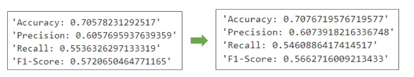
'Accuracy: 0.70578231292517'
'Precision: 0.6057695937639359'
'Recall: 0.5536326297133319'
'F1-Score: 0.5720650464771165'
import matplotlib.pyplot as plt
df_feature_importances_dt = pd.DataFrame({'Feature': X.columns, 'Importance': model_rf.feature_importances_})
df_feature_importances_dt = df_feature_importances_dt.sort_values(by='Importance', ascending=False).reset_index(drop=True)
display(df_feature_importances_dt)
Python
복사
Feature | Importance |
0 | begin_month |
1 | days_birth |
2 | income_total |
3 | days_employed |
4 | age |
5 | family_size |
6 | edu_type |
7 | reality |
8 | phone |
9 | car |
10 | child_num |
11 | gender |
12 | job_type_2 |
13 | job_type_4 |
14 | job_type_3 |
15 | work_phone |
16 | job_type_1 |
17 | email |
18 | income_type_1 |
19 | family_type_1 |
20 | family_type_2 |
21 | income_type_2 |
22 | house_type_2 |
23 | family_type_0 |
24 | house_type_1 |
25 | job_type_0 |
26 | house_type_0 |
27 | income_type_0 |
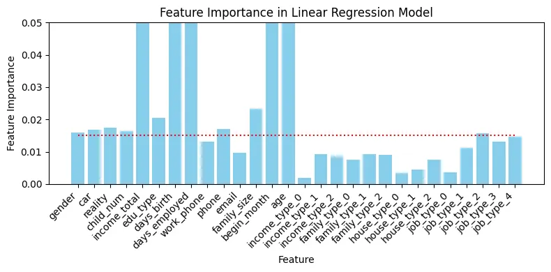
# 피처 중요도 시각화
low_importance_criteria = 0.015
ylimit_val = 0.05
# 피처 중요도를 수직 바 그래프로 시각화
fig, ax = plt.subplots(figsize=(8, 4))
ax.bar(X.columns, model_rf.feature_importances_, color='skyblue')
ax.hlines(low_importance_criteria, 0, len(X.columns)-1 , colors='r', linestyles='dotted', label='low criteria')
ax.set_xticks(range(len(X.columns))) # X축에 대한 틱 위치 설정
ax.set_xticklabels(X.columns, rotation=45, ha="right") # X축에 대한 레이블 설정
ax.set_xlabel("Feature") # X축 레이블
ax.set_ylabel("Feature Importance") # Y축 레이블
ax.set_ylim(0, ylimit_val) # Y축 범위
ax.set_title("Feature Importance in Linear Regression Model") # 그래프 제목 설정
plt.tight_layout()
plt.show()
Python
복사
# 특정 값 이하의 특성 중요도 갖는 피처 제거
low_feature_importances = df_feature_importances_dt[df_feature_importances_dt['Importance'] < low_importance_criteria]['Feature'].values.tolist()
Python
복사
# 검증 성능 변화 확인
# 피처 제거 후 성능 확인
train_credit_test1 = train_credit.copy()
X = train_credit_test1.drop(low_feature_importances + ['credit'], axis=1);
y = train_credit_test1['credit']
X_train, X_val, y_train, y_Val = train_test_split(X, y, test_size=0.20, random_state=42)
model_rf = RandomForestClassifier(random_state = 42)
model_rf.fit(X_train,y_train)
y_pred = model_rf.predict(X_val)
accuracy = accuracy_score(y_Val, y_pred)
precision = precision_score(y_Val, y_pred, average='macro')
recall = recall_score(y_Val, y_pred, average='macro')
f1 = f1_score(y_Val, y_pred, average='macro')
display(f'Accuracy: {accuracy}')
display(f'Precision: {precision}')
display(f'Recall: {recall}')
display(f'F1-Score: {f1}')
Python
복사
'Accuracy: 0.7076719576719577'
'Precision: 0.6073918216336748'
'Recall: 0.5460886417414517'
'F1-Score: 0.5662716009213433'

실전에서 피처 선택은 매우 신중하게 진행해야 한다.
바로 제거하기보다는 피처 변환, 생성 등의 피처 엔지니어링을 통해 타겟 변수와의 연관성이 높은 피처로 변환하거나 새로 생성하는 등의 노력이 필요하다.
또한, 한번의 검증 평가보다 교차 검증을 적용하는 것이 더 정확하다.